How to work in Excel. Creating formulas in Excel. Using text in formulas

In the second part of the Excel 2010 series for beginners, you will learn how to link table cells with mathematical formulas, add rows and columns to a ready-made table, learn about the AutoFill function, and much more.

Introduction

In the first part of the “Excel 2010 for Beginners” series, we got acquainted with the very basics of Excel, learning how to create regular tables in it. Strictly speaking, this is a simple matter and, of course, the capabilities of this program are much wider.

The main advantage of spreadsheets is that individual data cells can be linked together by mathematical formulas. That is, if the value of one of the interconnected cells changes, the data of the others will be recalculated automatically.

In this part, we will figure out what benefits such opportunities can bring using the example of the table of budget expenses that we have already created, for which we will have to learn how to create simple formulas. We will also get acquainted with the cell autofill function and learn how you can insert additional rows and columns into the table, as well as merge cells in it.

Perform basic arithmetic operations

In addition to creating regular tables, Excel can be used to perform arithmetic operations in them, such as addition, subtraction, multiplication and division.

To perform calculations in any table cell, you need to create inside it the simplest formula, which must always begin with an equal sign (=). To specify mathematical operations within a formula, ordinary arithmetic operators are used:

For example, let's imagine that we need to add two numbers - “12” and “7”. Place the mouse cursor in any cell and type the following expression: “=12+7”. When you have finished entering, press the “Enter” key and the cell will display the calculation result - “19”.

To find out what a cell actually contains - a formula or a number - you need to select it and look at the formula bar - the area located immediately above the column names. In our case, it just displays the formula that we just entered.

After carrying out all the operations, pay attention to the result of dividing the numbers 12 by 7, which is not an integer (1.714286) and contains quite a lot of digits after the decimal point. In most cases, such precision is not required, and such long numbers will only clutter the table.

To fix this, select the cell with the number for which you want to change the number of decimal places after the decimal point and on the tab home in Group Number select team Decrease bit depth. Each click on this button removes one character.

To the left of the team Decrease bit depth There is a button that performs the opposite operation - it increases the number of decimal places to display more accurate values.

Drawing up formulas

Now let's return to the budget table we created in the first part of this series.

At the moment, it records monthly personal expenses for specific items. For example, you can find out how much was spent on food in February or on car maintenance in March. But the total monthly expenses are not indicated here, although these indicators are the most important for many. Let's correct this situation by adding the line “Monthly expenses” at the bottom of the table and calculate its values.

To calculate the total expense for January in cell B7, you can write the following expression: “=18250+5100+6250+2500+3300” and press Enter, after which you will see the result of the calculation. This is an example of using a simple formula, the compilation of which is no different from calculations on a calculator. Unless the equal sign is placed at the beginning of the expression, and not at the end.

Now imagine that you made a mistake when indicating the values ​​of one or more expense items. In this case, you will have to adjust not only the data in the cells indicating expenses, but also the formula for calculating total expenses. Of course, this is very inconvenient and therefore in Excel, when creating formulas, not specific numerical values ​​are often used, but cell addresses and ranges.

With this in mind, let's change our formula for calculating total monthly expenses.

In cell B7, enter an equal sign (=) and... Instead of manually entering the value of cell B2, left-click on it. After this, a dotted highlight frame will appear around the cell, which indicates that its value is included in the formula. Now enter the “+” sign and click on cell B3. Next, do the same with cells B4, B5 and B6, and then press the ENTER key, after which the same amount value will appear as in the first case.

Select cell B7 again and look at the formula bar. It can be seen that instead of numbers - cell values, the formula contains their addresses. This is a very important point, since we just built a formula not from specific numbers, but from cell values ​​that can change over time. For example, if you now change the amount of expenses for purchasing things in January, then the entire monthly total expense will be recalculated automatically. Give it a try.

Now let's assume that you need to sum not five values, as in our example, but one hundred or two hundred. As you understand, using the above method of constructing formulas in this case is very inconvenient. In this case, it is better to use the special “AutoSum” button, which allows you to calculate the sum of several cells within one column or row. In Excel, you can calculate not only the sums of columns, but also rows, so we use it to calculate, for example, total food expenses for six months.

Place the cursor on an empty cell on the side of the desired line (in our case it is H2). Then click the button Sum on the bookmark home in Group Editing. Now, let's go back to the table and see what happened.

In the cell we selected, a formula appears with a range of cells whose values ​​need to be summed. At the same time, the dotted highlight frame appeared again. Only this time it frames not just one cell, but the entire range of cells, the sum of which needs to be calculated.

Now let's look at the formula itself. As before, the equals sign comes first, but this time it is followed by function“SUM” is a predefined formula that will add the values ​​of the specified cells. Immediately after the function there are brackets located around the addresses of the cells whose values ​​​​need to be summed, called formula argument. Please note that the formula does not indicate all the addresses of the cells being summed, but only the first and last ones. The colon between them indicates that range cells from B2 to G2.

After pressing Enter, the result will appear in the selected cell, but that’s all the button can do Sum don't end. Click on the arrow next to it and a list will open containing functions for calculating average values ​​(Average), the number of data entered (Number), maximum (Maximum) and minimum (Minimum) values.

So, in our table we calculated the total expenses for January and the total expenses on food for six months. At the same time, they did this in two different ways - first using cell addresses in the formula, and then using functions and ranges. Now, it's time to finish the calculations for the remaining cells, calculating the total costs for the remaining months and expense items.

Autocomplete

To calculate the remaining amounts, we will use one remarkable feature of Excel, which is the ability to automate the process of filling cells with systematic data.

Sometimes in Excel you have to enter similar data of the same type in a certain sequence, for example, days of the week, dates, or row numbers. Remember, in the first part of this series, in the table header, we entered the name of the month in each column separately? In fact, it was completely unnecessary to enter this entire list manually, since the application can do it for you in many cases.

Let's erase all the month names in the header of our table, except for the first one. Now select the cell labeled “January” and move the mouse pointer to its lower right corner so that it takes the form of a cross called fill marker. Hold down the left mouse button and drag it to the right.

A tooltip will appear on the screen, telling you the value the program is about to insert into the next cell. In our case, this is “February”. As you move the marker down, it will change to the names of other months, which will help you figure out where to stop. Once the button is released, the list will populate automatically.

Of course, Excel does not always correctly “understand” how to fill in subsequent cells, since the sequences can be quite diverse. Let's imagine that we need to fill a line with even numeric values: 2, 4, 6, 8 and so on. If we enter the number “2” and try to move the autofill marker to the right, it turns out that the program offers to insert the value “2” again both in the next and in other cells.

In this case, the application needs to provide a little more data. To do this, in the next cell on the right, enter the number “4”. Now select both filled cells and again move the cursor to the lower right corner of the selection area so that it takes the form of a selection marker. Moving the marker down, we see that the program has now understood our sequence and is showing the required values ​​in the tooltips.

Thus, for complex sequences, before using autofill, you need to fill in several cells yourself so that Excel can correctly determine the general algorithm for calculating their values.

Now let's apply this useful program feature to our table, so that we can enter formulas manually for the remaining cells. First, select the cell with the amount already calculated (B7).

Now “hook” the cursor on the lower right corner of the square and drag the marker to the right to cell G7. After you release the key, the application itself will copy the formula into the marked cells, while automatically changing the addresses of the cells contained in the expression, substituting the correct values.

Moreover, if the marker is moved to the right, as in our case, or down, then the cells will be filled in ascending order, and to the left or up - in descending order.

There is also a way to fill a row using tape. Let's use it to calculate the cost amounts for all expense items (column H).

We select the range that should be filled, starting from the cell with the data already entered. Then on the tab home in Group Editing press the button Fill and select the filling direction.

Add rows, columns, and merge cells

To get more practice in writing formulas, let's expand our table and at the same time learn a few basic formatting operations. For example, let’s add income items to the expenditure side, and then calculate possible budget savings.

Let's assume that the revenue part of the table will be located on top of the expenditure part. To do this we will have to insert a few extra lines. As always, this can be done in two ways: using commands on the ribbon or in the context menu, which is faster and easier.

Right-click in any cell of the second row and select the command from the menu that opens Insert…, and then in the window - Add line.

After inserting a row, pay attention to the fact that by default it is inserted above the selected row and has the format (cell background color, size settings, text color, etc.) of the row located above it.

If you need to change the default formatting, immediately after pasting, click the button Add Options icon that automatically appears near the lower right corner of the selected cell and select the option you want.

Using a similar method, you can insert columns into the table that will be placed to the left of the selected one and individual cells.

By the way, if a row or column ends up in the wrong place after insertion, you can easily delete it. Right-click on any cell belonging to the object to be deleted and select the command from the menu that opens Delete. Finally, indicate what exactly you want to delete: a row, a column, or an individual cell.

On the ribbon, you can use the button for adding operations Insert located in the group Cells on the bookmark home, and to delete, the command of the same name in the same group.

In our case, we need to insert five new rows at the top of the table immediately after the header. To do this, you can repeat the adding operation several times, or you can, having completed it once, use the “F4” key, which repeats the most recent operation.

As a result, after inserting five horizontal rows into the top part of the table, we bring it to the following form:

We left the white unformatted rows in the table on purpose to separate the income, expenditure and total parts from each other by writing appropriate headings in them. But before we do that, we will learn one more operation in Excel - merging cells.

When several adjacent cells are combined, one is formed, which can occupy several columns or rows at once. In this case, the name of the merged cell becomes the address of the uppermost cell of the merged range. At any time, you can split a merged cell again, but you cannot split a cell that has never been merged.

When merging cells, only the data in the top left is saved, but the data in all other merged cells will be deleted. Remember this and do the merging first, and only then enter the information.

Let's return to our table. In order to write headings in white lines, we need only one cell, while now they consist of eight. Let's fix this. Select all eight cells of the second row of the table and on the tab home in Group Alignment click on the button Combine and place in the center.

After executing the command, all selected cells in the row will be combined into one large cell.

Next to the merge button there is an arrow, clicking on which will bring up a menu with additional commands that allow you to: merge cells without central alignment, merge entire groups of cells horizontally and vertically, and also cancel the merge.

After adding headers, as well as filling out the lines: salary, bonuses and monthly income, our table began to look like this:

Conclusion

In conclusion, let's calculate the last line of our table, using the knowledge gained in this article, the cell values ​​of which will be calculated using the following formula. In the first month, the balance will be the normal difference between the income received for the month and the total expenses in it. But in the second month we will add the balance of the first to this difference, since we are calculating savings. Calculations for subsequent months will be carried out according to the same scheme - savings for the previous period will be added to the current monthly balance.

Now let's translate these calculations into formulas that Excel can understand. For January (cell B14) the formula is very simple and will look like this: “=B5-B12”. But for cell C14 (February), the expression can be written in two different ways: “=(B5-B12)+(C5-C12)” or “=B14+C5-C12”. In the first case, we again calculate the balance of the previous month and then add the balance of the current month to it, and in the second, the already calculated result for the previous month is included in the formula. Of course, using the second option to construct the formula in our case is much preferable. After all, if you follow the logic of the first option, then in the expression for the March calculation there will already be 6 cell addresses, in April - 8, in May - 10, and so on, and when using the second option there will always be three of them.

To fill the remaining cells from D14 to G14, we will use the ability to fill them automatically, just as we did in the case of amounts.

By the way, to check the value of the final savings for June, located in cell G14, in cell H14 you can display the difference between the total amount of monthly income (H5) and monthly expenses (H12). As you understand, they should be equal.

As can be seen from the latest calculations, in formulas you can use not only the addresses of adjacent cells, but also any others, regardless of their location in the document or belonging to a particular table. Moreover, you have the right to link cells located on different sheets of the document and even in different books, but we will talk about this in the next publication.

And here is our final table with the calculations performed:

Now, if you wish, you can continue filling it out yourself, inserting both additional items of expenses or income (rows) and adding new months (columns).

In the next article we will talk in more detail about functions, understand the concept of relative and absolute links, be sure to master several more useful elements of table editing, and much more.

The Microsoft Office Excel program is a table editor in which it is convenient to work with them in every possible way. Here you can also set formulas for basic and complex calculations, create graphs and diagrams, program, creating real platforms for organizations, simplifying the work of an accountant, secretary and other departments dealing with databases.

How to learn to work in excel on your own

The excel 2010 tutorial describes in detail the program interface and all the features available to it. To start working independently in Excel, you need to navigate the program interface, understand the taskbar, where commands and tools are located. To do this, you need to watch a lesson on this topic.

At the very top of Excel we see a ribbon of tabs with thematic sets of commands. If you move the mouse cursor over each of them, a tooltip appears detailing the direction of action.

Under the tab ribbon there is a “Name” line, where the name of the active element is written, and a “Formula line”, which displays formulas or text. When performing calculations, the “Name” line is converted into a drop-down list with a default set of functions. You just need to select the required option.

Most of the excel window is occupied by the work area, where tables, graphs are actually built, and calculations are made. . Here the user performs any necessary actions, using commands from the tab ribbon.

At the bottom of excel on the left side you can switch between workspaces. Additional sheets are added here if it is necessary to create different documents in one file. In the lower right corner there are commands responsible for convenient viewing of the created document. You can select the workbook viewing mode by clicking on one of the three icons, and also change the scale of the document by changing the position of the slider.

Basic Concepts

The first thing we see when opening the program is a blank sheet, divided into cells that represent the intersection of columns and rows. The columns are designated by Latin letters, and the rows by numbers. It is with their help that tables of any complexity are created and the necessary calculations are carried out in them.

Any video lesson on the Internet describes creating tables in Excel 2010 in two ways:

To work with tables, several types of data are used, the main of which are:

• text,
• numerical,
• formula.

By default, text data is aligned to the left of cells, and numeric and formula data is aligned to the right.

To enter the desired formula into a cell, you need to start with the equal sign, and then by clicking on the cells and putting the required signs between the values ​​​​in them, we get the answer. You can also use the drop-down list with functions located in the upper left corner. They are recorded in the “Formula Bar”. It can be viewed by making a cell with a similar calculation active.

VBA to excel

The programming language built into the Visual Basic for Applications (VBA) application makes it easier to work with complex data sets or repetitive functions in Excel. Programming instructions can be downloaded on the Internet for free.

In Microsoft Office Excel 2010, VBA is disabled by default. In order to enable it, you need to select “Options” in the “File” tab on the left panel. In the dialog box that appears, on the left, click “Customize Ribbon”, and then on the right side of the window, check the box next to “Developer” so that such a tab appears in Excel.

When starting to program, you need to understand that an object in Excel is a sheet, workbook, cell and range. They obey each other, so they are in a hierarchy.

Application plays a leading role . Next come Workbooks, Worksheets, Range. Thus, you need to specify the entire hierarchy path to access a specific cell.

Another important concept is properties. These are the characteristics of objects. For Range it is Value or Formula.

Methods represent specific commands. They are separated from the object by a dot in VBA code. Often when programming in Excel, the Cells (1,1) command is needed. Select. In other words, you need to select a cell with coordinates (1,1), that is, A 1.

It can greatly facilitate the user’s work with tables and numerical expressions by automating it. This can be achieved using the application's tools and its various functions. Let's look at the most useful of them.

Due to the wide functional purpose of the program, the user is not always aware of the capabilities that simplify interaction with many Excel tools. Later in the article, we will talk about the 10 best functions that can be useful for various purposes, and also provide links to detailed lessons on working with each of them.

VLOOKUP function

One of the most requested features in Microsoft Excel is "VLOOKUP". By using it, you can drag and drop values ​​from one or more tables into another. In this case, the search is performed only in the first column of the table, thus, when the data in the source table is changed, data is automatically generated in the derived table, in which individual calculations can be performed. For example, information from a table containing price lists for goods can be used to calculate indicators in the table about the volume of purchases in monetary terms.

A VLOOKUP is started by inserting a statement "VPR" from "Function Masters" in the cell where the data should be displayed.

In the window that appears, after running this function, you need to specify the address of the cell or range of cells from which the data will be pulled.

Pivot tables

Another important function of Excel is the creation of pivot tables, which allows you to group data from other tables according to various criteria, perform various calculations with them (summation, multiplication, division, etc.), and the results are displayed in a separate table. At the same time, there are very wide possibilities for customizing the fields of the pivot table.

It is created on the tab "Insert" by pressing the button, which is called - "Pivot table".

Creating Charts

To visually display data placed in a table, it is convenient to use charts. They are often used for creating presentations, writing scientific papers, for research purposes, etc. Excel provides a wide range of tools for creating various types of charts.

To create a chart, you need to select a set of cells containing the data that you want to visually display. Then, while on the tab "Insert", select on the ribbon the type of diagram that you consider most suitable for achieving your goals.

More precise setup of charts, including setting its name and axes names, is done in the group of tabs "Working with diagrams".

One type of chart is graphs. The principle of their construction is the same as that of other types of diagrams.

Formulas in Excel

To work with numerical data, the program allows you to use special formulas. With their help, you can perform various arithmetic operations with data in tables: addition, subtraction, multiplication, division, exponentiation, root extraction, etc. To apply the formula, you need to put the sign in the cell where you plan to display the result «=» . After this, the formula itself is entered, which can consist of mathematical symbols, numbers and cell addresses. To indicate the address of the cell from which the data for calculation is taken, just click on it with the mouse, and its coordinates will appear in the cell for displaying the result.

Excel is also convenient to use as a regular calculator. To do this, in the formula bar or in any cell, simply enter mathematical expressions after the sign «=» .

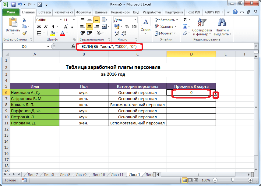
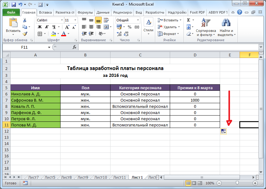
"IF" function

One of the most popular functions used in Excel is "IF". It makes it possible to specify in a cell the output of one result if a specific condition is met and another result if it is not met. Its syntax is as follows: IF(boolean expression; [result if true]; [result if false]) .

Operators "AND", "OR" and nested function "IF" matches several conditions or one of several conditions.

Macros

Using macros, the program records the execution of certain actions, and then they are played back automatically. This significantly saves time on performing a large amount of the same type of work. Macros are recorded by enabling the capture of your actions in the program through the corresponding button on the ribbon.

Macros can also be recorded using the Visual Basic markup language in a special editor.

Conditional Formatting

To highlight specific data, a table uses conditional formatting to set rules for highlighting cells. The conditional formatting itself can be done in the form of a histogram, color scale, or set of icons. You can access it through the tab "Home" highlighting the range of cells you are going to format. Next in the tools group "Styles" click the button named "Conditional Formatting". After this, all you have to do is select the formatting option that you consider most suitable.

The formatting will be completed.

Smart table

Not all users know that a table simply drawn with a pencil or borders is perceived by Excel as a simple area of ​​cells. You can force the program to see this data set as a table through reformatting. This is done simply: first, select the desired range with data, and then, being on the tab "Home", click on the button "Format as table". A list will appear with various design style options, where you can select the one that suits you.

The table is also created by clicking the button "Table", which is located on the tab "Insert", having previously selected a certain area of ​​the sheet with data.

The editor will treat the selected set of cells as a table. As a result, for example, if you enter some data into the cells located at the borders of the table, they will be automatically included in it. In addition to this, when scrolling down, the header will be constantly within the field of view.

Parameter selection

Using the parameter selection function, you can select the initial data, guided by the result you want. Go to the tab "Data" and press the button "What If Analysis" located in the toolbox "Working with data". In the list that appears, select the item “Selection of parameter...”.

The parameter selection window will open. In field "Set in cell" you must provide a reference to the cell that contains the formula you want. In field "Meaning" the end result you want must be specified. In field "Changing cell values" insert the coordinates of the cell with the value being adjusted.

INDEX function

Features the function provides "INDEX", somewhat close to the capabilities of the function "VPR". It also allows you to search for data in an array of values ​​and return it to a specified cell. The syntax is as follows: INDEX(cell_range, row_number, column_number) .

This is not a complete list of all the functions that are available in Microsoft Excel. We focused only on the most popular and most important of them.

Excel is one of the most powerful applications in the entire Office suite. It is used not only by accountants and economists, but also by ordinary people. The program is designed to work with numbers and tables, making it possible to present information in the most convenient form for perception: as charts and graphs. Here you can carry out complex calculations and perform various mathematical operations. In addition, the user does not need special knowledge; it is enough to learn how to work in Excel.

What is this office application?

Excel works with files that form a kind of book consisting of separate sheets. Letters, symbols and numbers are entered into table cells. They can be copied, moved or deleted. If necessary, various operations are carried out with them: text, mathematical, logical and others. Beginners who are just learning how to work in Excel should know that any information can be displayed on the screen in the form of graphs or charts.

How to create a file?

First of all, you need to open the document. To create it, you need to click on the program shortcut or go to the application through “Start”.

By default, the name is “Book 1,” but you can enter any name in the “File name” line. While working, you should periodically save data to avoid loss of information in the event of a computer crash or freeze.

You can easily switch between sheets by clicking on the corresponding inscription at the bottom of the page. If there are a lot of tabs, it is better to use the arrows on the keyboard. To insert a sheet, you need to find the “Insert” item in the “Home” menu. It will display all the possible actions that apply to the sheets, such as adding or deleting. Tabs can also be moved.

"Face" of the program

Before you figure out how to work in Excel, it’s worth studying the interface. The tools are located at the top and bottom of the window, and the rest of the area is occupied by rectangles, which are cells. The peculiarity of spreadsheets is that actions can be performed in some cells, and the result can be displayed in others.

Each table has columns that are designated by letters of the English alphabet. Lines are numbered on the left. Thus, any cell has its own coordinates. You can enter both data and formulas in each cell. Before entering the latter, you must put the “=” symbol.

Each cell has its own characteristic

To understand how to learn to work in Excel correctly, the user must know that before entering values, it is necessary to set the dimension of the column or cell. It will depend on how the data is measured. To do this, right-click on the selected range and select “Format Cells” in the dialog box.

If the entered number is greater than 999, you must set the division by digits. You should not enter spaces yourself.

To display data correctly, you cannot enter more than one individual value in one cell. Also, do not enter enumerations separated by commas or other characters. Each value must have its own cell.

How to enter data?

Users who know will have no problem entering data. To do this, you need to click on the cell and type letters or numbers on the keyboard. To continue working, you must press “Enter” or TAB. Line breaks are performed using the ALT + “ENTER” combination.

When entering a month or number in order, just enter the value in the initial cells, and then drag the marker to the required range.

Wrap text

Most often, users are interested in learning how to work with text in Excel. If necessary, it can be word-hyphenated. To do this, you need to select certain cells and in the “Home” tab you need to find the “Alignment” option, and then select “Text Wrap”.

If you want to automatically change the width and height of a cell according to the entered text, you should do the following: go to the “Home” tab and select “Format” in the “Cells” group. Next you need to select the appropriate action.

Formatting

To format numbers, you need to select the cell and find the “Number” group in the “Home” tab. After clicking on the arrow next to the “General” item, you can select the required format.

To change the font, you need to select a specific range and go to the “Home” menu, “Font”.

How to create a table?

Knowledge of how to work in Excel is unlikely to be useful to a user if he does not know how to create a table. The easiest way is to highlight a specific range and mark the boundaries with black lines by clicking on the corresponding icon at the top of the page. But often a non-standard table for forms or documents is required.

First of all, you need to decide what the table should look like in order to set the width and length of the cells. Having selected the range, you need to go to the “Format Cells” menu and select “Alignment”. The “Merge Cells” option will help remove unnecessary borders. Then you need to go to the “Borders” menu and set the required parameters.

Using the Format Cells menu, you can create different table options by adding or removing columns and rows, and changing borders.

Knowing how to work in an Excel table, the user will be able to create headings. To do this, in the “Table Formatting” window, you need to check the box next to the “Table with headers” item.

To add elements to a table, you must use the Design tab. There you can select the required parameters.

What are macros for?

If a user has to frequently repeat the same actions in a program, knowledge of how macros work in Excel will be useful. They are programmed to perform actions in a certain sequence. Using macros allows you to automate certain operations and alleviate monotonous work. They can be written in different programming languages, but their essence does not change.

To create a macro in this application, you need to go to the “Tools” menu, select “Macro”, and then click “Start Recording”. Next, you need to perform those actions that are often repeated, and after finishing the work, click “Stop recording”.

All these instructions will help a beginner figure out how to work in Excel: keep records, create reports and analyze numbers.

Good afternoon.

Once upon a time, writing a formula in Excel on my own was something incredible for me. And even despite the fact that I often had to work in this program, I didn’t type anything except text...

As it turned out, most of the formulas are not complicated and can be easily worked with, even by a novice computer user. In this article, I would like to reveal the most necessary formulas with which you most often have to work...

So, let's begin…

1. Basic operations and basics. Excel basics training.

All actions in the article will be shown in Excel version 2007.

After launching the Excel program, a window appears with many cells - our table. main feature The program is that it can calculate (like a calculator) your formulas that you write. By the way, you can add a formula to each cell!

The formula must begin with the “=” sign. This is a must. Next, you write what you need to calculate: for example, “=2+3” (without quotes) and press the Enter key - as a result, you will see that the result “5” appears in the cell. See screenshot below.

Important! Despite the fact that the number “5” is written in cell A1, it is calculated using the formula (“=2+3”). If you simply write “5” in the next cell, then when you hover the cursor over this cell, in the formula editor (the line at the top, Fx) - you will see the prime number “5”.

Now imagine that in a cell you can write not just the value 2+3, but the numbers of the cells whose values ​​​​need to be added. Let’s say “=B2+C2”.

Naturally, there must be some numbers in B2 and C2, otherwise Excel will show us a result equal to 0 in cell A1.

And one more important note...

When you copy a cell that has a formula in it, for example A1 - and paste it into another cell - it is not the value “5” that is copied, but the formula itself!

Moreover, the formula will change in direct proportion: i.e. if A1 is copied to A2, then the formula in cell A2 will be “=B3+C3”. Excel automatically changes your formula: if A1=B2+C2, then it is logical that A2=B3+C3 (all numbers increased by 1).

The result, by the way, is in A2=0, because Cells B3 and C3 are not specified, which means they are equal to 0.

This way, you can write the formula once, and then copy it to all the cells of the desired column - and Excel itself will perform the calculation in each row of your table!

If you don't want B2 and C2 to change when copying and have always been linked to these cells, then simply add a “$” sign to them. Example below.

This way, no matter where you copy cell A1, it will always refer to the linked cells.

2. Adding values ​​in rows (SUM and SUMIFS formula)

You can, of course, add each cell, making the formula A1+A2+A3, etc. But to avoid this hassle, there is a special formula in Excel that will add up all the values ​​in the cells that you select!

Let's take a simple example. There are several items of goods in stock, and we know how many of each product separately in kg. In stock. Let's try to calculate how much is in kg. cargo in warehouse.

To do this, go to the cell in which the result will be shown and write the formula: “=SUM(C2:C5)”. See screenshot below.

As a result, all cells in the selected range will be summed, and you will see the result.

2.1. Addition with condition (with conditions)

Now let’s imagine that we have certain conditions, i.e. You don’t need to add up all the values ​​in the cells (Kg, in stock), but only certain ones, say, with a price (1 kg) less than 100.

There is a wonderful formula for this “ SUMIFS". Immediately an example, and then an explanation of each symbol in the formula.

=SUMIFS(C2:C5,B2:B5,“<100» ) , Where:

C2:C5 - the column (those cells) that will be summed up;

B2:B5- column against which the condition will be checked (i.e. price, for example, less than 100);

«<100» - the condition itself, please note that the condition is written in quotes.

There is nothing complicated in this formula, the main thing is to maintain proportionality: C2:C5;B2:B5 - correct; C2:C6;B2:B5 - incorrect. Those. The sum range and the condition range must be proportional, otherwise the formula will return an error.

Important! There can be many conditions for the amount, i.e. You can check not by the 1st column, but by 10 at once, setting many conditions.

3. Counting the number of rows that satisfy the conditions (COUNTIFS formula)

A fairly common task: to count not the sum of values ​​in cells, but the number of such cells that satisfy certain conditions. Sometimes there are a lot of conditions.

So, let's begin.

To count goods in the required cell, write the following formula (see above):

=COUNTIFS(B2:B5,“>90”), Where:

B2:B5- the range by which they will check, according to the condition we set;

">90"- the condition itself is enclosed in quotation marks.

Now let’s try to complicate our example a little and add an invoice for one more condition: with a price greater than 90 + quantity in stock less than 20 kg.

The formula takes the form:

=COUNTIFS(B2:B6,”>90″,C2:C6 ;“<20» )

Here everything remains the same, except for one more condition ( C2:C6;"<20″ ). By the way, there can be a lot of such conditions!

It is clear that no one will write such formulas for such a small table, but for a table of several hundred rows this is a completely different matter. As an example, this table is more than clear.

4. Search and substitution of values ​​from one table to another (VLOOKUP formula)

Let's imagine that we received a new table with new price tags for the goods. It’s good if there are 10-20 items, you can “refill” them all manually. What if there are hundreds of such names? It would be much faster if Excel independently found matching names from one table to another, and then copied the new price tags into our old table.

For such a problem, the formula is used VLOOKUP. At one time I was playing tricks with logical formulas “IF” until I came across this wonderful thing!

So, let's begin…

Here is our example + a new table with price tags. Now we need to automatically substitute new price tags from the new table into the old one (new price tags are red).

Place the cursor in cell B2 - i.e. to the first cell where we need to change the price tag automatically. Next, we write the formula as in the screenshot below (after the screenshot there will be a detailed explanation of it).

=VLOOKUP(A2 ;$D$2:$E$5 ;2 ), Where

A2- the value that we will look for in order to take a new price tag. In our case, we are looking for the word “apples” in the new table.

$D$2:$E$5- select our new table completely (D2:E5, selection goes from the upper left corner to the lower right diagonally), i.e. where the search will take place. The “$” sign in this formula is necessary so that when copying this formula to other cells - D2:E5 does not change!

Important! The word "apples" will be searched only in the first column of your selected table; in this example, "apples" will be searched in column D.

2 - When the word “apples” is found, the function must know from which column of the selected table (D2:E5) to copy the desired value. In our example, copy from column 2 (E), because in the first column (D) we performed the search. If your selected table for search consists of 10 columns, then the first column is searched, and from columns 2 to 10 you can select a number to copy.

To formula =VLOOKUP(A2,$D$2:$E$5,2) substituted new values ​​for other product names - just copy it to other cells of the column with product price tags (in our example, copy to cells B3:B5). The formula will automatically search and copy the value from the column you need in the new table.

5. Conclusion

In this article we looked at the basics of working with Excel, starting with how to start writing formulas. They gave examples of the most common formulas that most people who work in Excel often have to work with.

I hope that the analyzed examples will be useful to someone and will help speed up their work. Happy experimenting!

What formulas do you use? Is it possible to somehow simplify the formulas given in the article? For example, on weak computers, when changing some values ​​in large tables where calculations are made automatically, the computer freezes for a couple of seconds, recalculating and showing new results...